Custom Grid Editor (CG)

This module enables you to create and edit custom 2-dimensional initialization grids for the 2-dimensional spectrum analysis.

• Custom grids can be defined by varying two if the attributes listed and fixing one (sedimentation coefficient, frictional ratio, molecular weight, vbar and diffusion coefficient).

• It is also possible to define multiple grid regions and combine them into a single grid which defines multiple solute regions.

• The custom grid can be re-displayed in the other domains left unchanged.

Note

It is also possible to define grids that contain both sedimenting and floating species, in which case the grid needs to be defined for a fixed frictional ratio, but permits variations in vbar to account for the difference in buoyancy while maintaining positive molecular weights.

• All combined partial grids are saved as a special model structure that can be stored in the database or on disk to be submitted with either the desktop or supercomputing version of the 2-dimensional spectrum analysis.

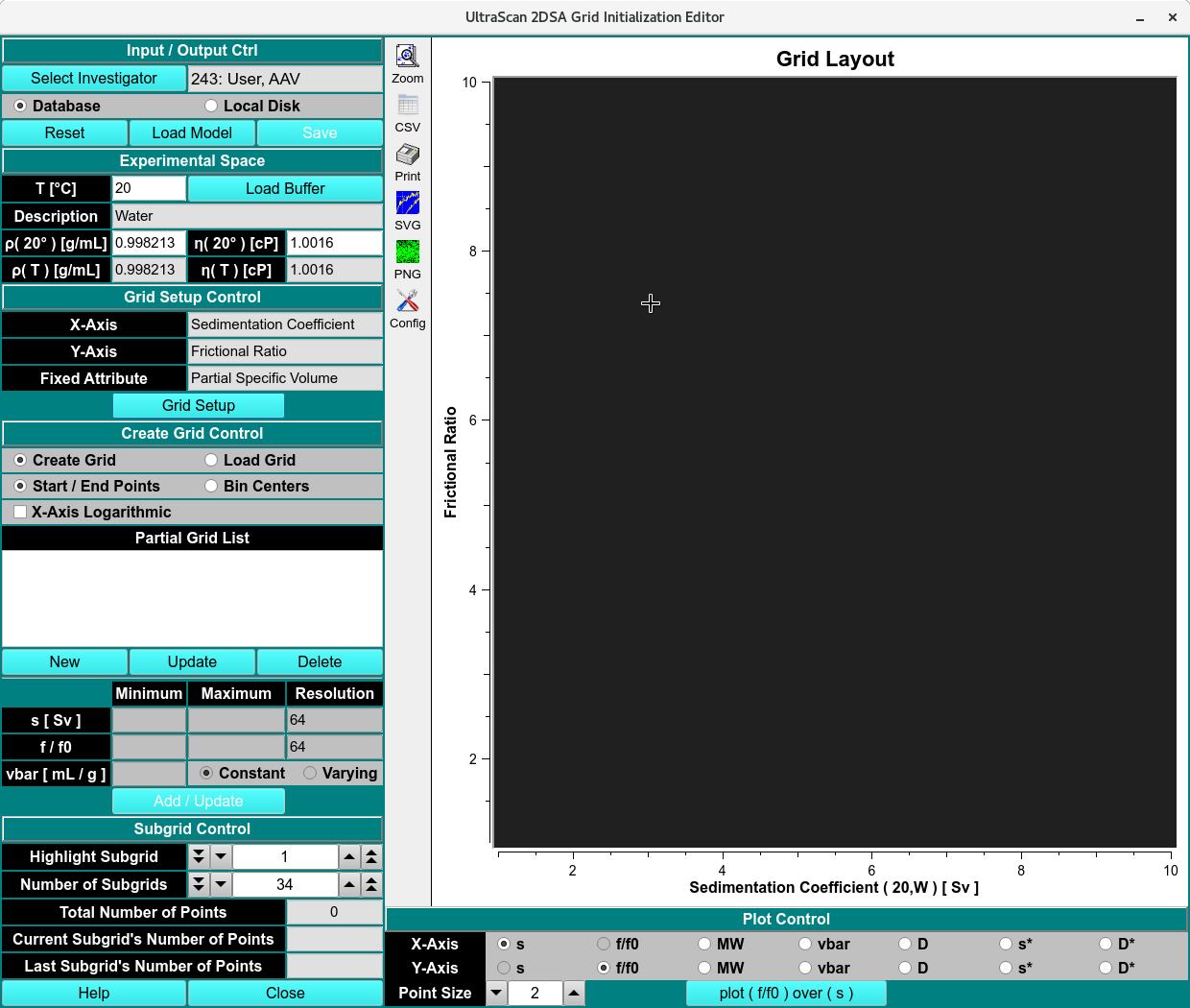
Custom Grid Editor - Create Model

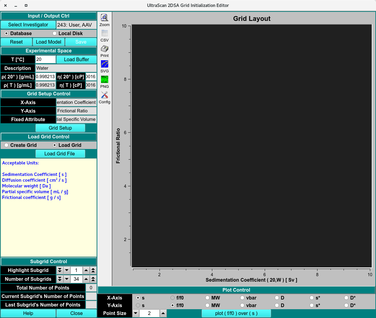
Custom Grid Editor - Load Model

Processes:

Create a Grid

1. Select the investigator to save the model to or from.

2. Click Load Buffer to define the experimental parameters of the dataset by loading the buffer used. Once selected the density and viscosity of the buffer will populate the Description, Density (ρ) and Viscosity (η) at 20°C and the selected temperature.

3. Under the Grid Setup Controls, select the two variable attributes and one fixed attribute.

4. Select Create Grid radio button and prerequisite the grid by picking Start/End Points or bin centers to start the grid points at the edge of bin or center.

Note

For unevenly distributed samples over a large s range, the x attribute can be spaced logarithmically clicking X-Axis Logarithmic. This is typically done for samples with aggregates.

5. To add a partial grid to the list, click New and the X and Y attribute minimum, maximum and resolution boxes will be available to edit.

6. Select Constant for the Fixed Attribute or Varying if prior information is available. Varying the fixed Attribute will create a 3-D box or line, for best results, contact Ultrascan-III Development Team

7. Repeat steps 5-7 for every partial grids needed.

8. Once the grid is created, the Current Subgrid’s Number of Points must be ≤ 150. Increase or decrease Number of Subgrids to adjust Current Subgrid’s Number of Points to the right value and a diffusely spaced subgrid (displayed as Yellow dots).

Note

Each subgrid should be small enough to fit into the computer memory of the analysis program. The more subgrids are defined, the more grids will need to be calculated. If sufficient cores are available, this could speed up the analysis, but it will also lead to increasingly inefficient use of the available cores as there will be CPU-idling in the later stages of the analysis when the outputs of multiple grids are merged.

9. Once the grid has been created, click Save and a Save Grid Model dialog will appear to edit name and save.

View or Edit an Existing Grid

Note

Users cannot change the grid setup for existing grids.

1. Select the investigator to load the model from.

2. Click Load Model to call Load Distribution Model dialog and Accept. The selected model grid will populate the Grid plot.

3. From the Partial Grid List, select the grid to edit and click Update or Delete. This will to enable the grayed out area.

4. Adjust the values of the X and Y attributes and click Add/Update.

5. Once the grid has been edited, click Save and a Save Grid Model dialog will appear to edit name and save.

Functions:

Input/Output Controls

Select Investigator	Click here to retrieve the investigator management widget.
Database/Local Disk	Select the data target. If Database is selected, the model will be stored in the database. This is required if submitting a supercomputing job for the custom grid. Local Disk will only save the grid to the local disk for use in the desktop version of the 2-dimensional spectrum analysis.

Experimental Space

T [C]	The temperature selected by the user in the Buffer Management module. Manually setting the temperature will readout arbitrary Value!!! error.
Load Buffer	Load the buffer using the Buffer Management module.
Description	Read out the buffer selected or error if temperature is not set in the buffer management module.
p (20°C) [g/mL]	The density value is set by default to those of water at 20°C.
n (20°C) [cP]	The viscosity value are set by default to those of water at 20°C.
p (T°C) [g/mL]	The density value set by user.
n (T°C) [cP]	The viscosity value set by user.

Note

The density and viscosity values are set by default to those of water at 20°C. This means that all hydrodynamics variables are adjusted to standard conditions, which is what the analysis routines expect on input.For academic purposes, it is possible to change these values to see what the resulting grids look like. Under normal circumstances these values should never be adjusted.

Grid Setup Control

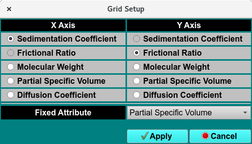
Custom Grid Editor - Grid Setup Dialog

X-Axis	Displays the selected X-Axis attribute.
Y-Axis	Displays the selected Y-Axis attribute.
Fixed Attribute	Displays the selected fixed attribute.
Grid Setup	Click to choose the X-Axis, Y-Axis and fixed attributes.

Create Setup Control

Create Grid	Radio button to call all the functions required to create a grid as show above.
Load Grid	Radio button to call all the functions required to load a pre-existing grid as show above.
Start / End Points	Select to start and end the grid points on the integer of the X and Y Axis attributes.
Bin Centers	Select to start and end the grid points on the middle of the X and Y Axis attribute integers.
Partial Grid List	List of the grids made.
New	Create new subgrid.
Update	Update and edit existing subgrid.
Delete	Delete existing subgrid.
Minimum and Maximum controls:	use these controls to adjust the minimum and maximum of the grid dimension. The labels will change according to the choice for X and Y dimensions.
Resolution	these controls allow you to set the grid resolution for any partial grid in both the X and Y dimensions. The label on these controls will change according to the selected X and Y dimensions, i.e., s-value or Mol. Weight Resolution:. The grid resolution should be high enough to cover the resolution contained in the experimental data. Excessive resolution will significantly increase the computational cost, without any appreciable benefit in goodness of fit. A too coarse resolution will not produce a good fit. If you see obvious step functions in the model that do not trace the underlying data well then you likely are not using sufficient resolution in your grid.
Constant	Keep the fixed attribute constant.
Varying	Vary the fixed attribute in the Set Z-Value Function
Add/Update	Apply and merge the grid parameters to total grid model.

Grid Spacing:

The parameter are required to be spaced evenly, and should not exclude major regions of the search space. Below are examples of Good and Bad grid spaceing.

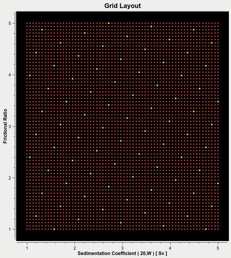
Good Spacing

Bad Spacing

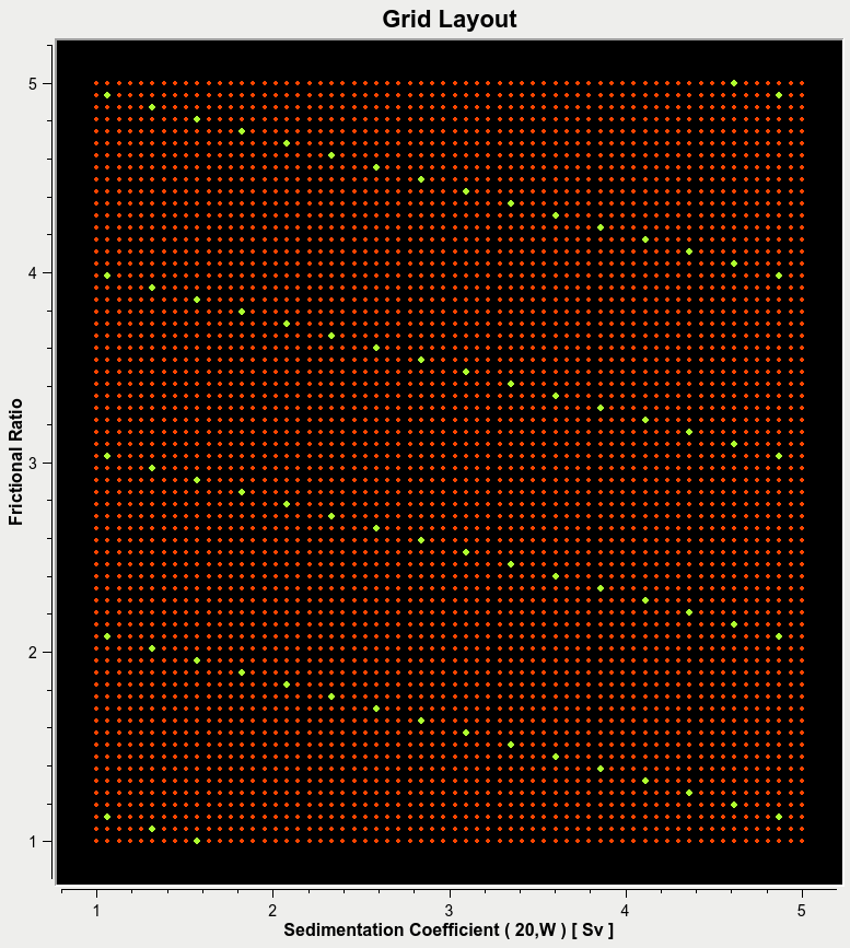
Example of custom grid spacing

Subgrid Control

Highlight Subgrid	Highlight one of the total subgrids.
Number of Subgrids	The total number of subgrids. The number can be increased or decreased depending on computational availability or need, See .
Total Number of Points	Number of subgrids X Number of points per subgrid
Current Subgrid’s Number of Points	The number of points in current subgrid.
Last Subgrid’s Number of Points	The number of points in the last subgrid.
Help	Software documentation for the custom grid module.
Close	Close the window.

Plot Control

X-Axis and Y-Axis	these controls are used to switch between views of the defined grid. A rectangular grid may be defined in the sedimentation domain, which looks like this when displayed with the molecular weight view.
Point Size	Size of the points.
plot ( ) over ( )	Revert to the rectangular grid.

Set Z-Value Function:

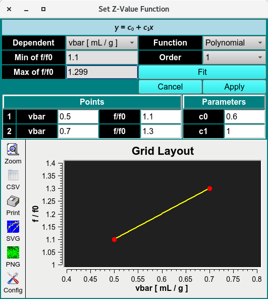
Set Z-Value Function

The Set Z-Value Function (advanced control) in the Custom Grid module lets users vary the third variable using predefined Z-Value Dependency Function equations. These equations constrain the third attribute as a function of one of the two variable attributes, using prior information to define the relationship.

Dependent	The variable attribute the third attribute will be constrained to.
Min of (Fixed)	The minimum value of the Dependent.
Max of (Fixed)	The maximum value of the Dependent.
Function	Select between polynomial or exponential functions.
Order	Select the order of the polynomial functions (1-5).
Fit	Fit the function and function parameters enters.
Cancel	Cancel Fit.
Apply	Apply the fitted function to the main window.
Grid Points	Enter the interval of the x and y attributes
Grid Parameters	Enter the partial concentration of the x and y attributes
Grid Layout	Plot the function and parameters selected.