Parametrically Constrained Spectrum Analysis

This module enables you to perform parametrically constrained spectrum analysis on a chosen experimental data set. Upon completion of an analysis fit, plots available include: model lines; experiment; simulation; overlayed experiment and simulation; residuals; time-invariant noise; radially-invariant noise; 3-D model. Final outputs may include a model and computed noises.

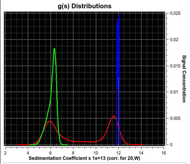
The PCSA method is used for composition analysis of sedimentation velocity experiments. It can generate sedimentation coefficient, diffusion coefficient, frictional coefficient, f/f0 ratio, and molecular weight distributions. The distributions can be plotted as 3-dimensional plots (2 parameters from the above list against each other), with the third dimension representing the concentration of the solute found in the composition analysis. The set of all such final calculated solutes form a model which is used to generate a simulation via Lamm equations. The simulation is plotted overlaying a plot of experimental data.

The PCSA pass proceeds for a set of models each of which consists of the solute points along a curve in s, f/f0 space. The model whose RMSD of the resulting residuals (simulation-experimental difference) is the lowest forms the starting point for a second phase which uses Levenberg-Marquardt to refine the model to a final output model. The set of initial curves is specified by a s and f/f0 ranges and a direct or implied number of variations in f/f0 end-points or sigmoid par1, par2 values. The type of curve used may be any of the following.

• Straight Line

• Increasing Sigmoid

• Decreasing Sigmoid

• Horizontal Line [C(s)]

Overview of PCSA Process:

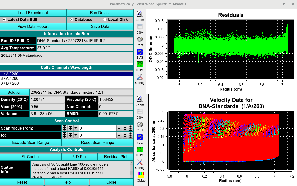
1. Load Experimental Data: First, load experimental velocity data. Click on “Load Data” to select an edited velocity data set from the database or from local disk.

2. Define the Analysis Fit: Secondly, open an analysis control window by clicking on “Fit Control”. Within that dialog, define the ranges and counts that comprise the analysis.

3. Start the Fit: Next, after having specified analysis parameters, begin the fit analysis by clicking “Start Fit”.

4. Display and Save Results: After simulation, a variety of options are available for displaying simulation results, residuals, and distributions. Report text files and graphics plot files can also be generated.

PCSA Simulated Data

The Curves:

After specifying the curve type and the variations to analyze, a plot of the model lines may be displayed.

Envelope and Combined Displays

PCSA Function

Straight Lines	Increasing Sigmodial	Decreasing Sigmodial	Horizontal Line (C(s))