Protocol Development

Allows for analysis profile optimization by re-attaching GMP runs at the LIMS Import stage with a modified Aprofile

Manage Optima Runs:

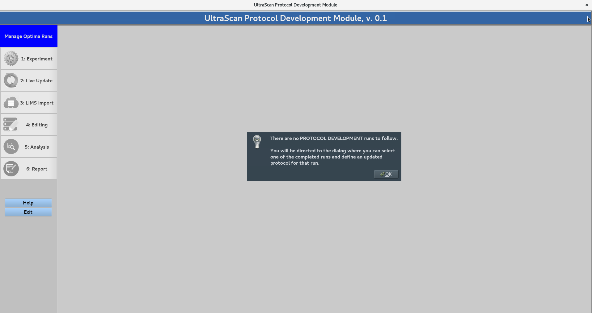
Select Completed Autoflow Run:

Provides a list of completed GMP runs in the database, as well as the current reporting stage (Report generation or collection of e-signatures).

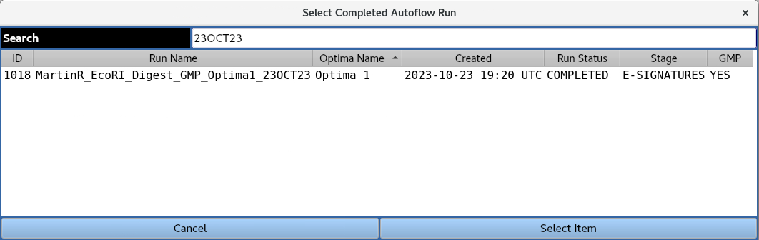
A GMP run can be loaded from the database by highlighting it and clicking the Select Item button. This opens a modified Data Acquisition Routine, where the user can assign a new protocol name. However, the run name and experimental parameters cannot be changed, as the run is being reimported for editing and analysis.

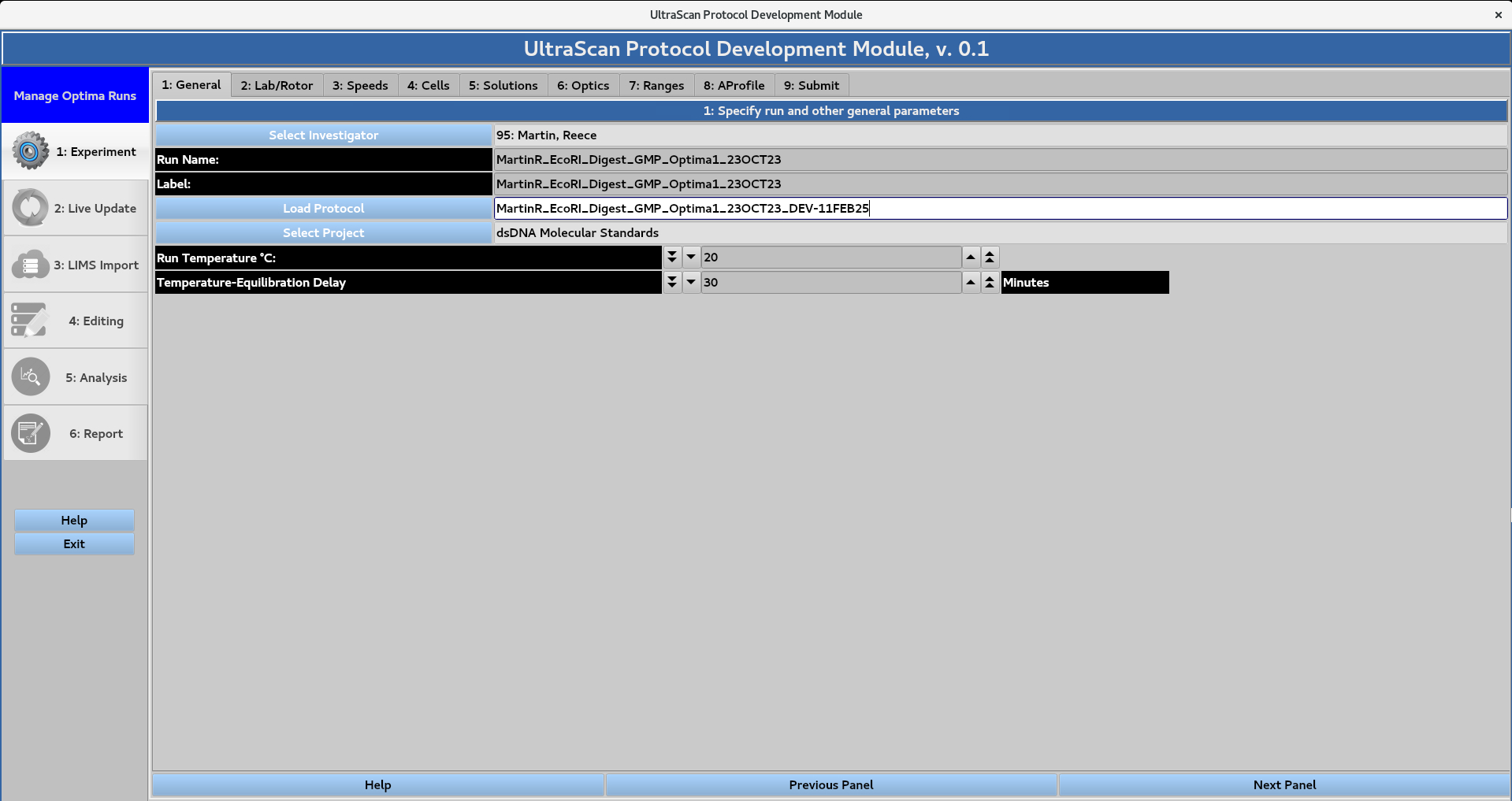
Sections 1-9 can be accessed in any order using the navigation bar at the top of the window or sequentially using the Previous Panel and Next Panel buttons at the bottom of the window.

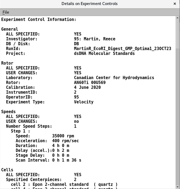
1: General

The protocol name is the only information that can be changed, since the source GMP run (Run Name, Label, Run Temperature and Temperature-Equilibration Delay) remains unchanged.

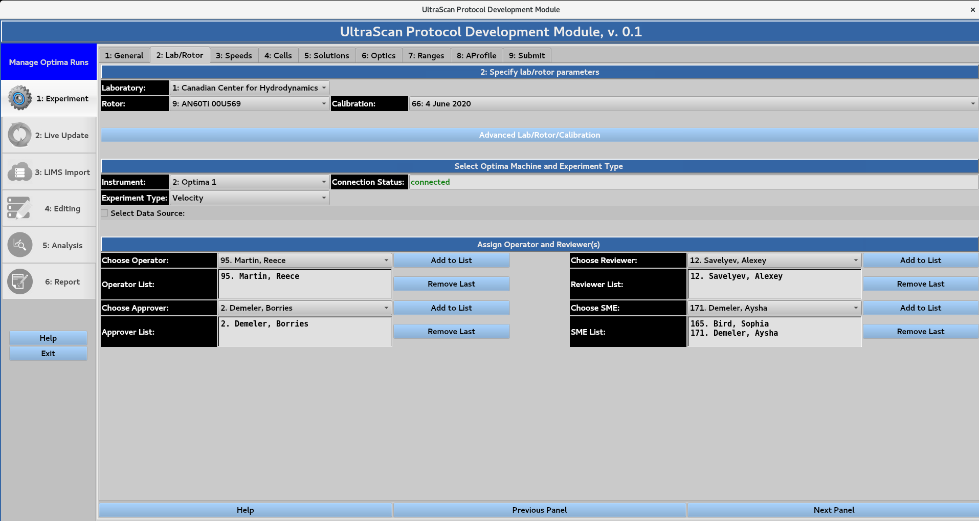
2: Lab/Rotor

The user cannot change the laboratory, rotor, rotor calibration profile, instrument, and experiment types. The roles of Operator, Reviewer, Approver, and Subject Matter Expert (SME) can be re-assigned from the drop-down menus. See here for more information: UltraScan GMP Help.

3: Speeds

None of the run parameters in this window can be modified.

4: Cells

None of the run parameters in this window can be modified.

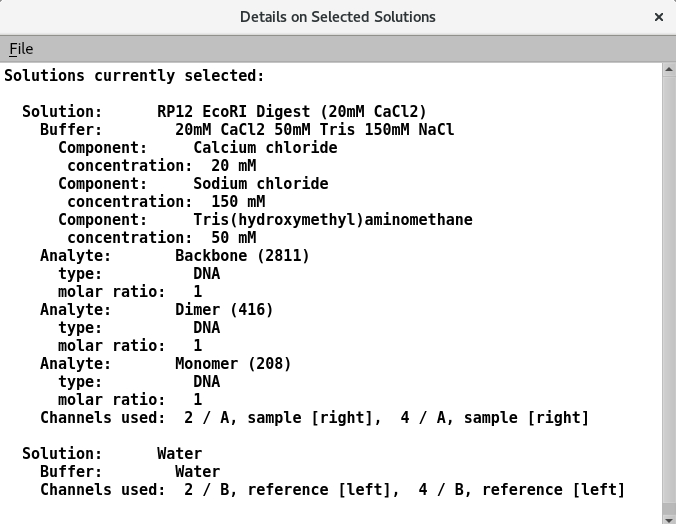
5: Solutions

None of the run parameters in this window can be modified.

5b: Solution Details

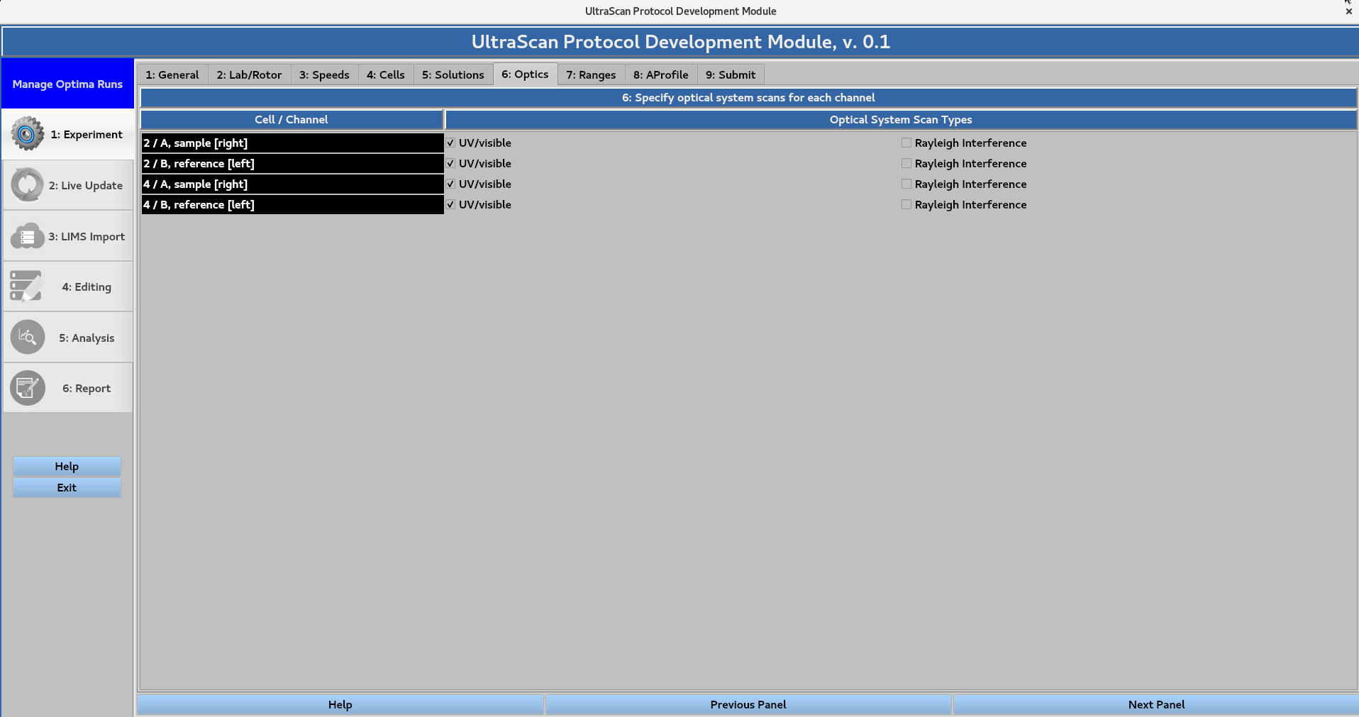
6: Optics

None of the run parameters in this window can be modified.

7: Ranges

None of the run parameters in this window can be modified.

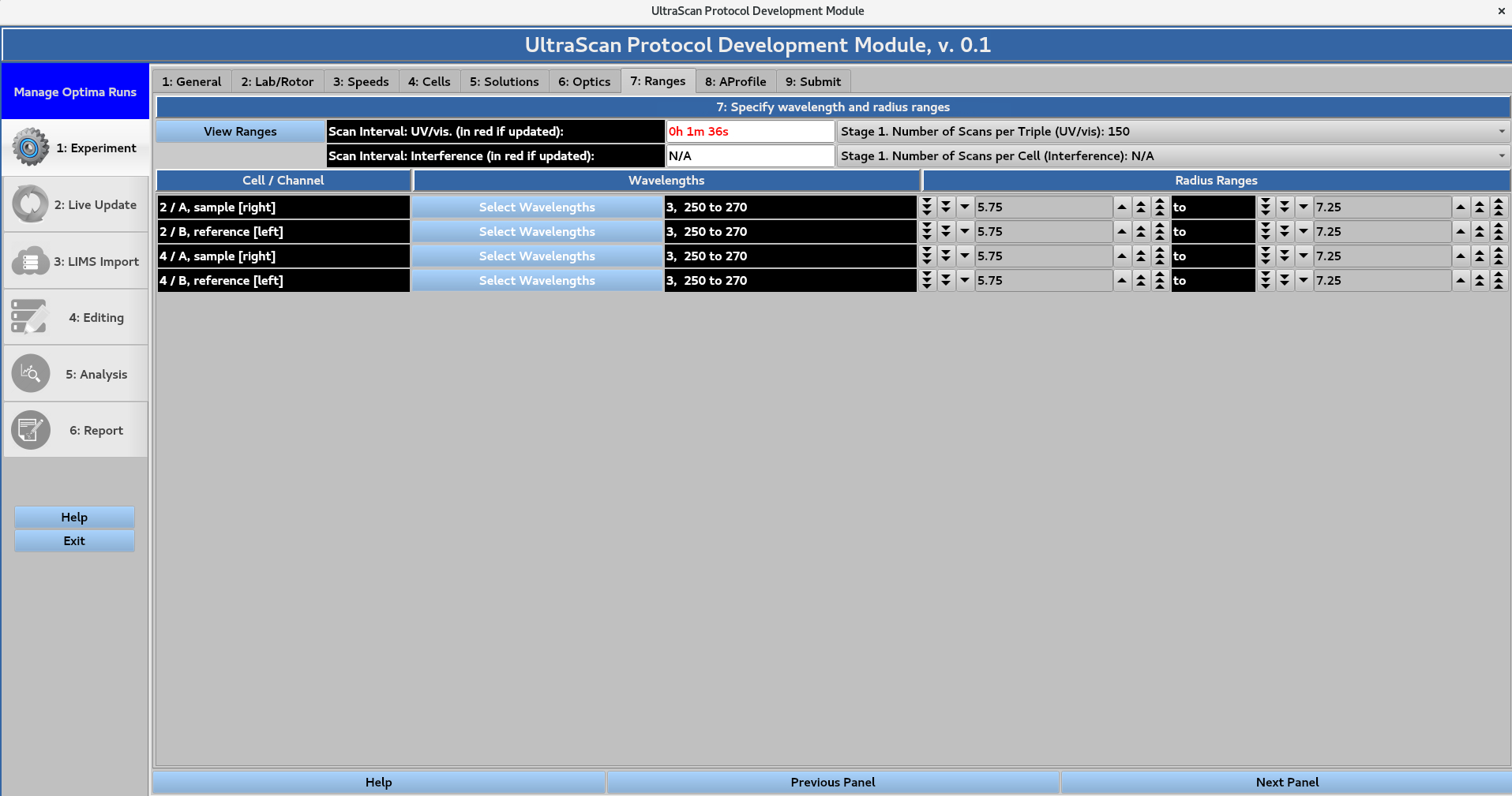
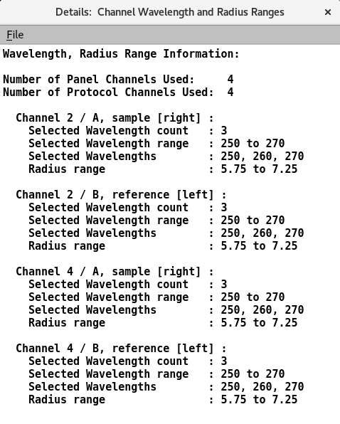
7a: View Ranges

8: AProfile (Analysis Profile)

Define edit profiles, analysis parameters and report settings for the experiment.

8.1: General

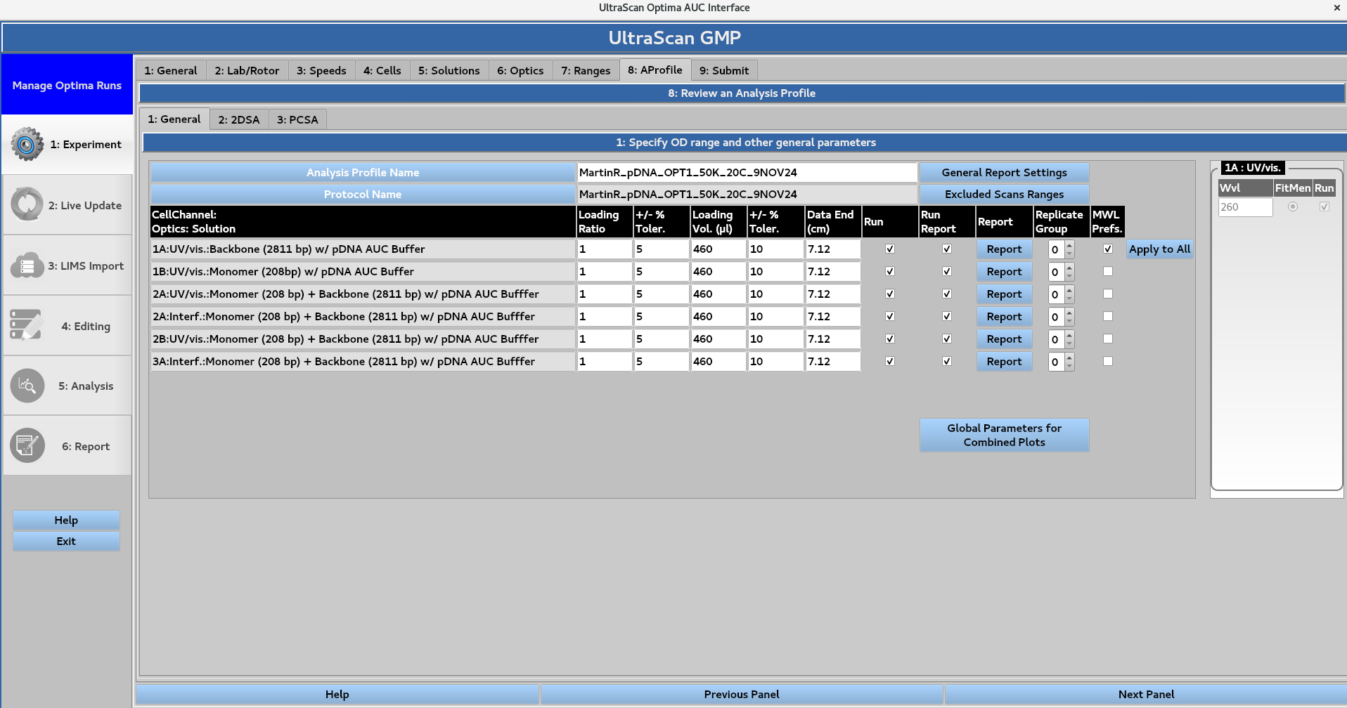
Define numerical values for ‘Loading Ratio’, the ‘± %Tolerance’, ‘Loading Volume (μL)’, the ‘± %Tolerance’, and ‘Data End (cm)’. The user can then select checkboxes to specify whether the analysis should be ‘Run’, and included in the ‘Run Report’.

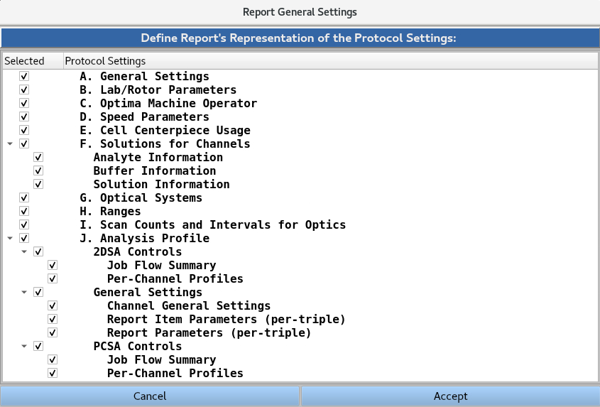
The Report General Settings windows allow the user to select/deselect which of the protocol settings (Sections 1-8) will be presented in the report. The {down arrow} button can be used to collapse or expand each subsection.

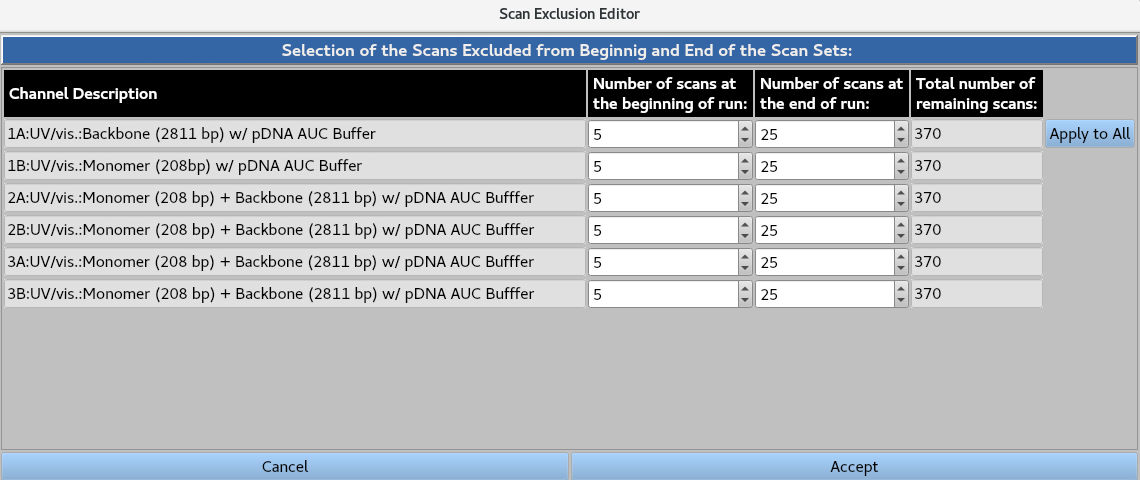
The Scan Exclusion Editor allows the user to numerically define the number scans to be removed from the beginning and end of each channel, either by typing the value or using the arrows. The Apply to All button applies the values for the first channel to all channels.

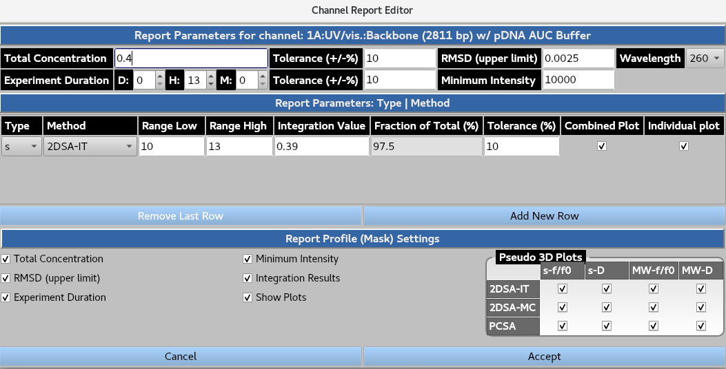
The Report button summons the channel-specific report settings window. The user defines the ‘Total Concentration’, the ‘ ± %Tolerance’, ‘RMSD (upper limit)’, the ‘± %Tolerance’, and the wavelength to extract these metrics from. The user then lists the expected ‘Experiment Duration’, the ‘± %Tolerance’, and ‘Minimum Intensity’ at the selected wavelength from the xenon flash lamp that is deemed acceptable. In the ‘Report Profile (Mask) Settings’ the user can select the following: ‘Total Concentration’, ‘Minimum Intensity’, ‘RMSD (upper limit)’, ‘Integration Results’, ‘Experiment Duration’ and relevant plots (as well as the pseudo-3D plots for each parameter and analysis type) they wish to be included in the report.

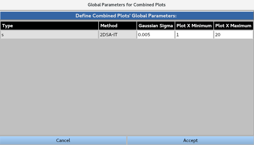
Global Parameters for Combined Plots allows the user to define the plot minimum, plot maximum and Gaussian sigma for each plot type.

8.2: 2DSA

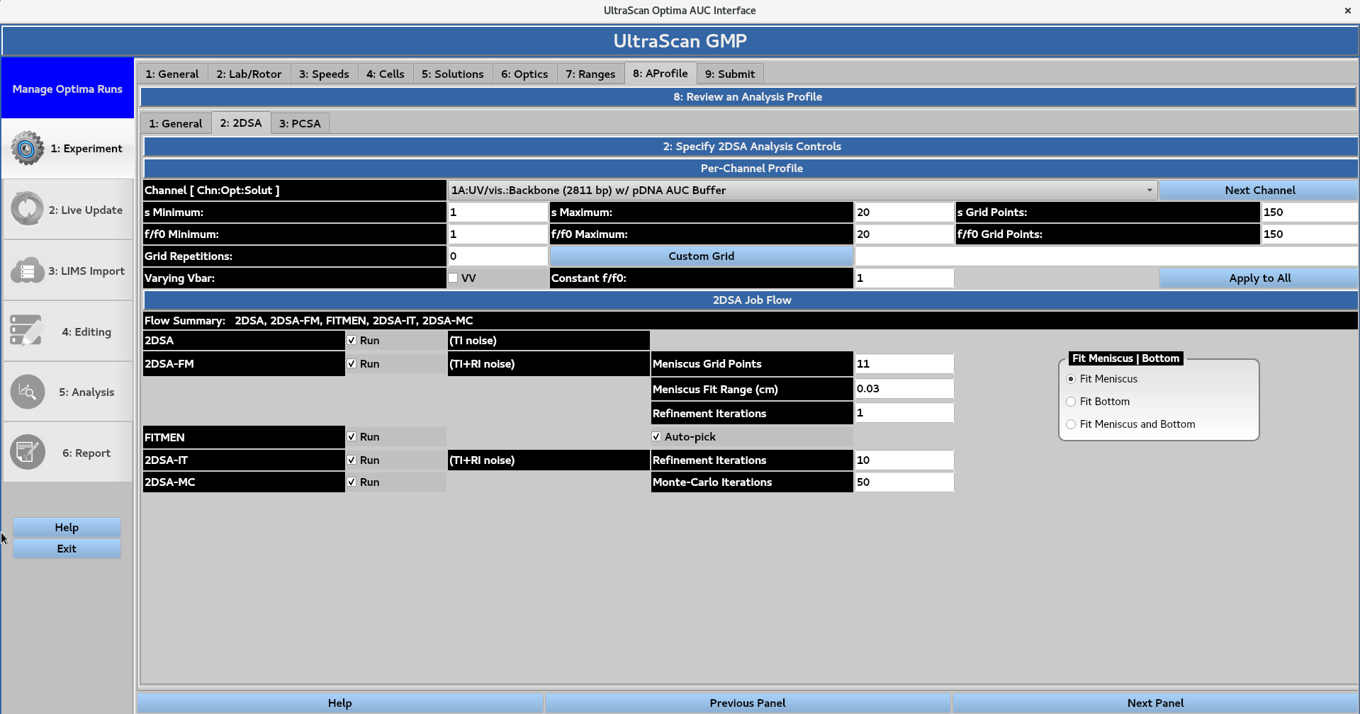
The user can define the 2-dimensional spectrum analysis (2DSA) controls for each channel. The grid size is defined by the minimum and maximum values for the sedimentation coefficient (<em>s</em>) and frictional ratio (<em>f/f0</em>), while the grid resolution is defined by the number of points for each of the parameters. A 2DSA Custom Grid (CG) can also be used if the user requires higher resolution in certain regions of the data, and only needs lower resolution in other regions. The user can also select to vary the partial specific volume or ‘Vbar’ parameter and hold the frictional ratio constant at a specified value. The Apply to All button can be used to apply these settings to all of the channels.

The ‘2DSA Job Flow’ panel allows the user to control which analysis steps are performed, including:

• 2DSA

• 2DSA with meniscus fit (FM), with a user-defined number of grid points, range (cm), and number of refinement iterations. The user can also choose to fit only the bottom of the channel or both the meniscus and the bottom.

• FITMEN meniscus processing, with the option to ‘Auto-pick’ the meniscus position

• 2DSA with iterative refinement (IT), with a user-defined number of iterations

• 2DSA with Monte Carlo iterations (MC), with a user-defined number of Monte Carlo iterations.

8.3: PCSA

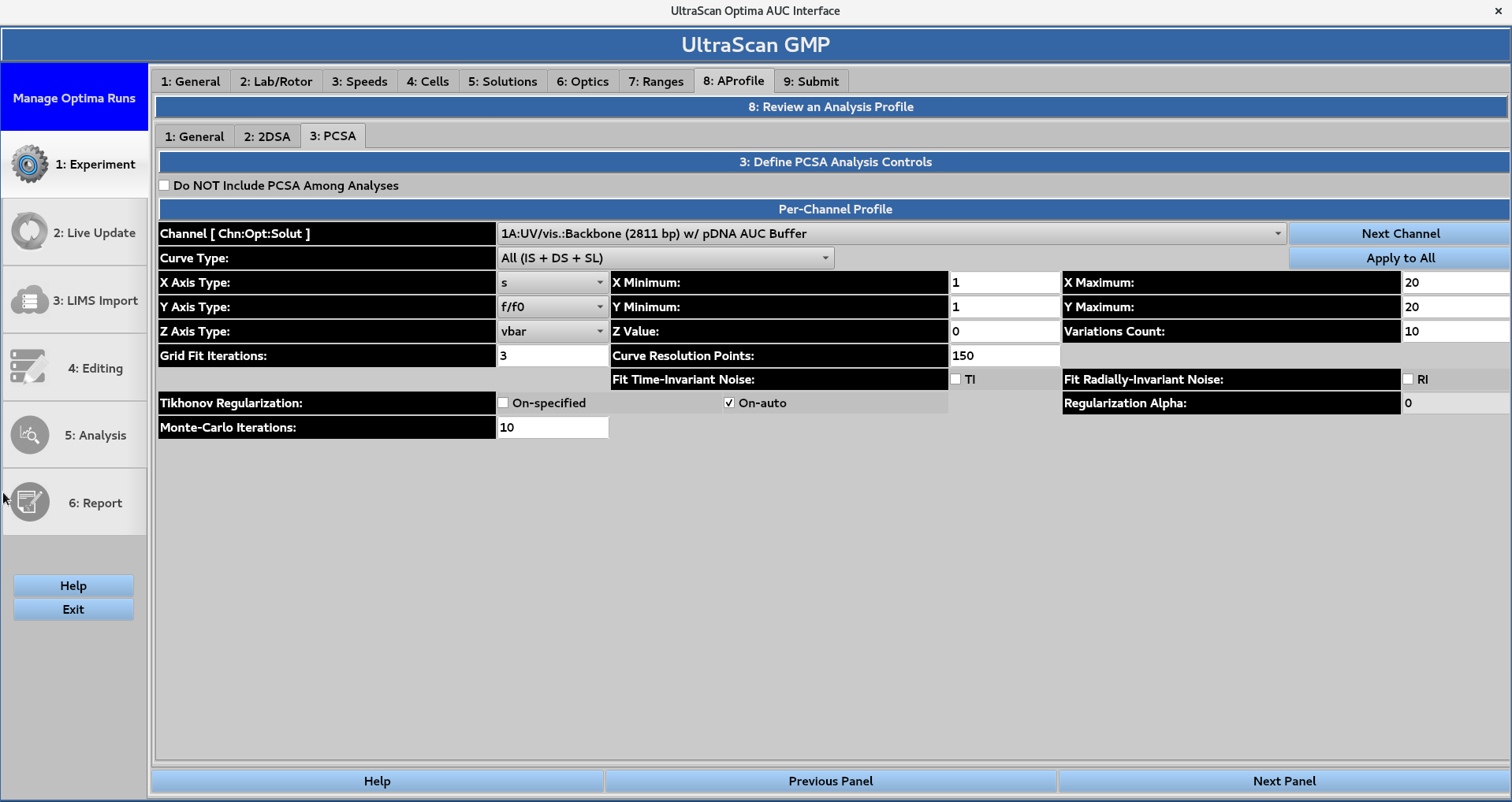
The user can select the option to not include the parametrically-constrained spectrum analysis (PCSA) in the submitted jobs. If the box is left unchecked, the user can define the PCSA controls for each channel.

The desired curve type is selected from the drop-down menu, and the user defines parameters for the x, y, and z axes.

• The x and y axes are defined by minimum and maximum values

• The z axis is assigned a value and a variation count

• Numerical values are then assigned for the grid fit iterations and curve resolution points

Optional settings include:

• Time- and radially-invariant noise fitting

• Tikhonov regularization, with either an auto-picked or manually-selected alpha

• Number of Monte Carlo iterations.

The ‘Apply to All’ button can be used to apply these parameters and settings to all of the channels.

9: Submit

Submit the protocol development run for processing

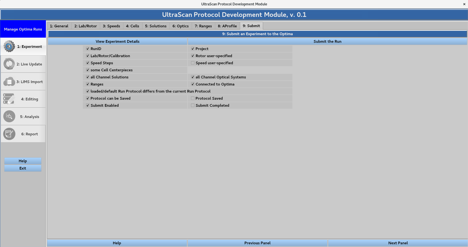
9a: View Experiment Details

Summary of the information defined in sections 1-8.

9b: Submit the Run

A new protocol name and GMP e-signer roles must be assigned before the ‘Submit the Run’ button becomes active and allows for submission. Submission prompts the following window:

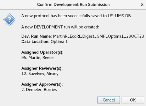
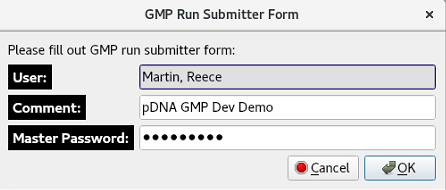
The ‘OK’ button prompts the ‘GMP Run Submitter Form’, allowing the user to add a comment and prompting them for their master password for authentication.

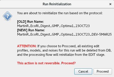
The ‘OK’ button brings up the ‘Run Reinitialization’ window, which informs the user that ‘Proceed’ will delete existing edit profiles, models, and noises, and reinitialize at the EDIT stage.

The program moves to the ‘IMPORT’ stage, which displays the last scan of each triple from the intensity data. The user is prompted with the Reference Scans: Automated Processing message:

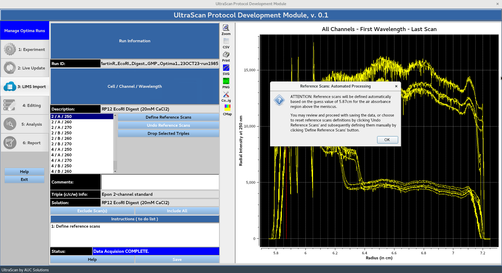
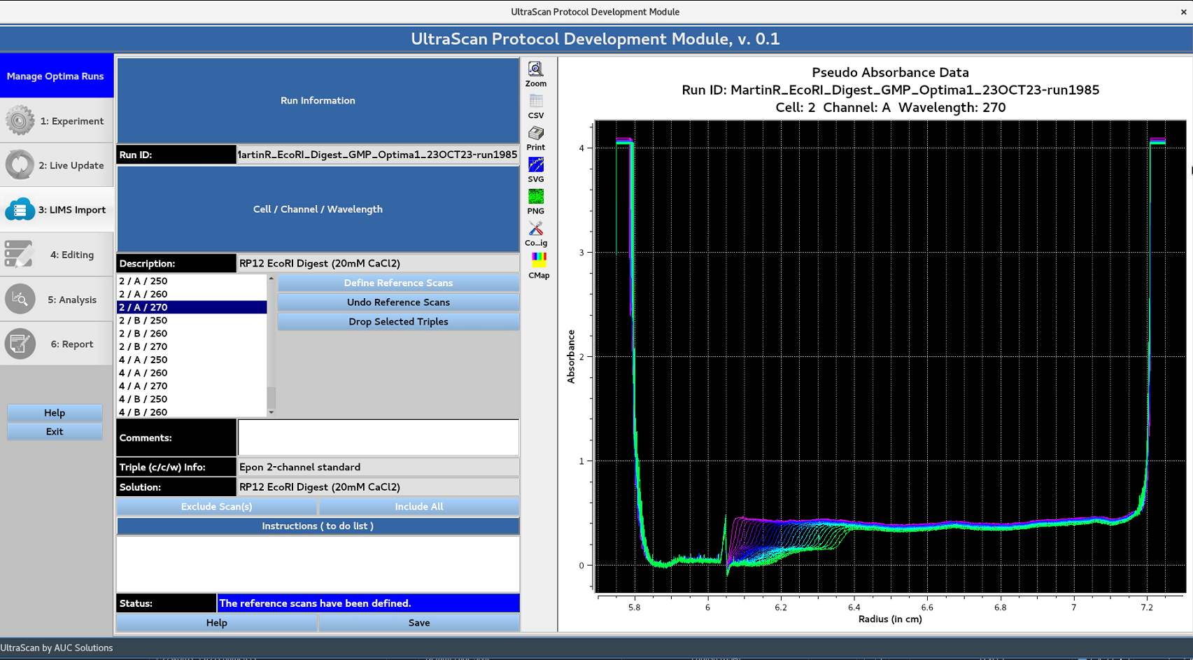
Clicking OK displays the converted absorbance data following the automated reference scan processing. If the user is not satisfied with the automated reference scans processing, the Undo Reference Scans button allows for them to be defined manually using the Define Reference Scans button. Drop Selected Triples can be used to drop unwanted triples.

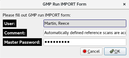
The Save button prompts the GMP Run IMPORT Form, allowing the user to add a comment and prompting them for their master password for authentication.

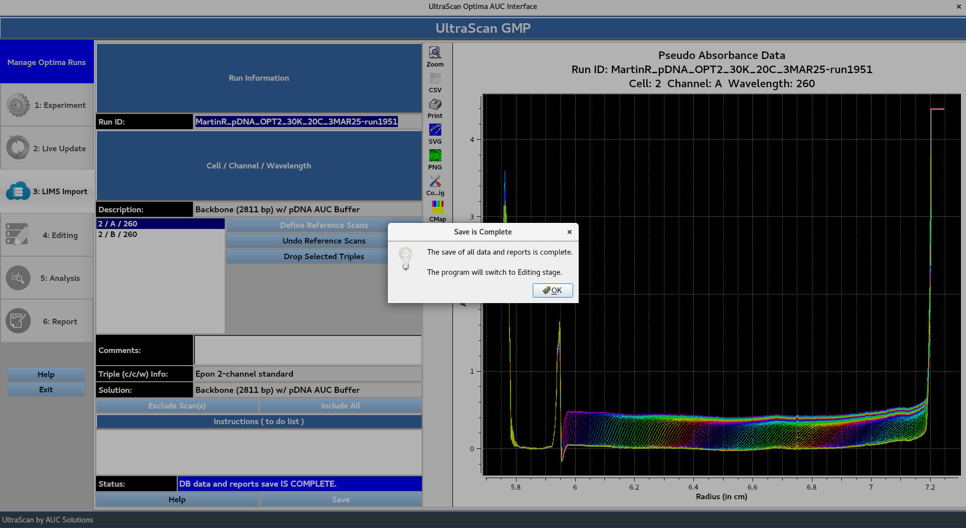
Once the data has been saved, the user is notified that the program is proceeding to the editing stage:

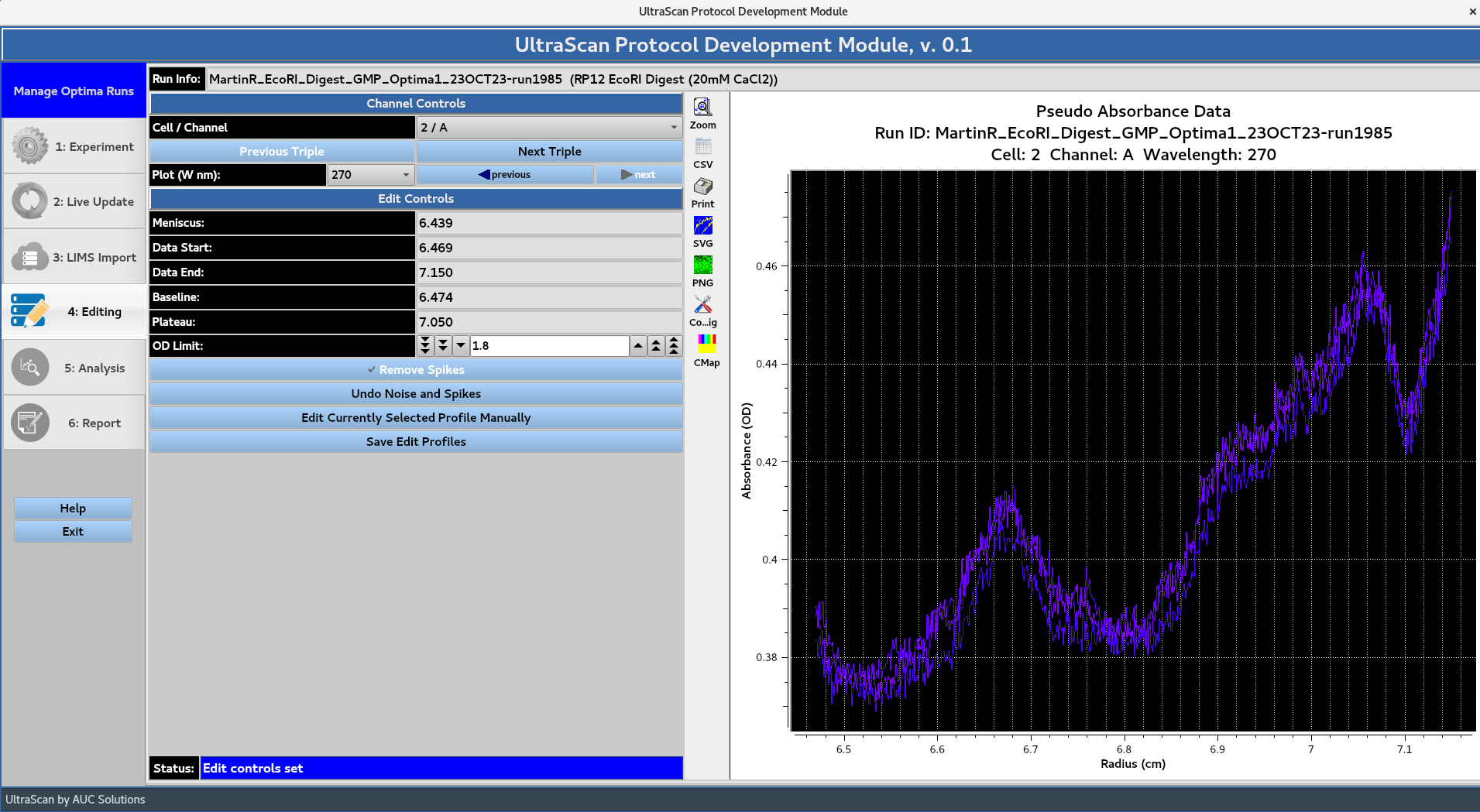
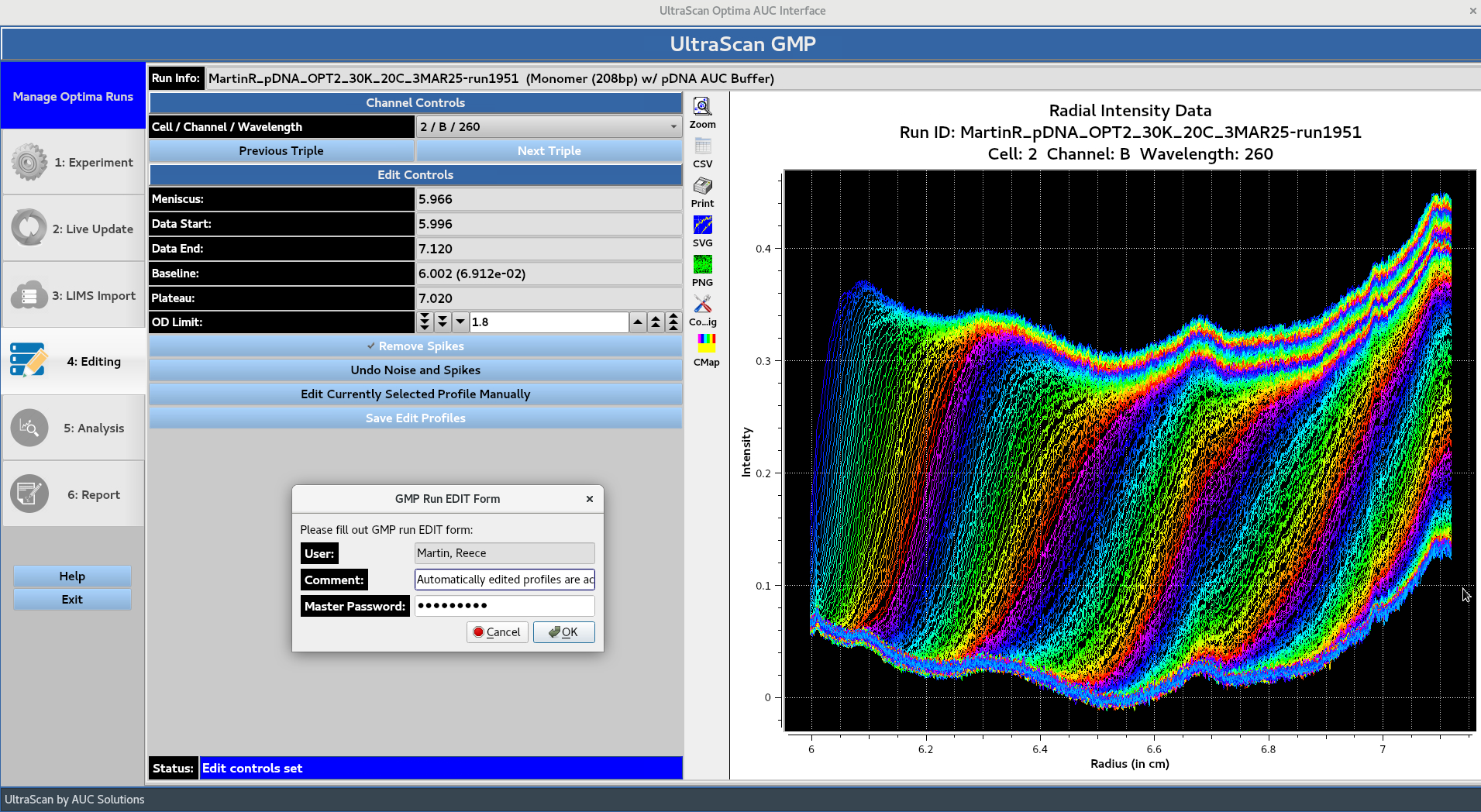
The editing window presents the user with the data edited in accordance with ‘Data End’ value and ‘Excluded Scan Ranges’ defined in the Aprofile. The ‘Meniscus’ position and ‘Data Start’ value are defined through automated processing. If the user is not satisfied with the automated processing, the Edit Currently Selected Profile Manually button allows for the ‘Meniscus’ position and ‘Data End’ values to be defined manually. Remove Spikes removes some sharp, irregular intensity spikes from data. Each cell/channel/wavelength triple can be cycled through using the Previous Triple and Next Triple buttons.

The Save Edit Profiles button prompts the GMP Run EDIT Form, allowing the user to add a comment and prompting them for their master password for authentication.

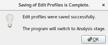
Once the edited profiles have been saved, the user is notified that the program is proceeding to the analysis stage:

The analysis window displays the current status of the submitted jobs producing the models specified in the Aprofile. Cancel can be used to stop ongoing jobs. View Fit simulates completed model overlays and displays them. The Expand All Triples and Collapse All Triples buttons control all triples, while the {down arrow} button can be used to collapse or expand each individual triple.

Once the analysis stage is complete, the models are simulated and the report is built. Which prompts the Report Generation Complete message box.

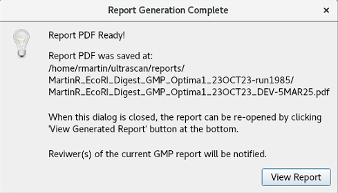
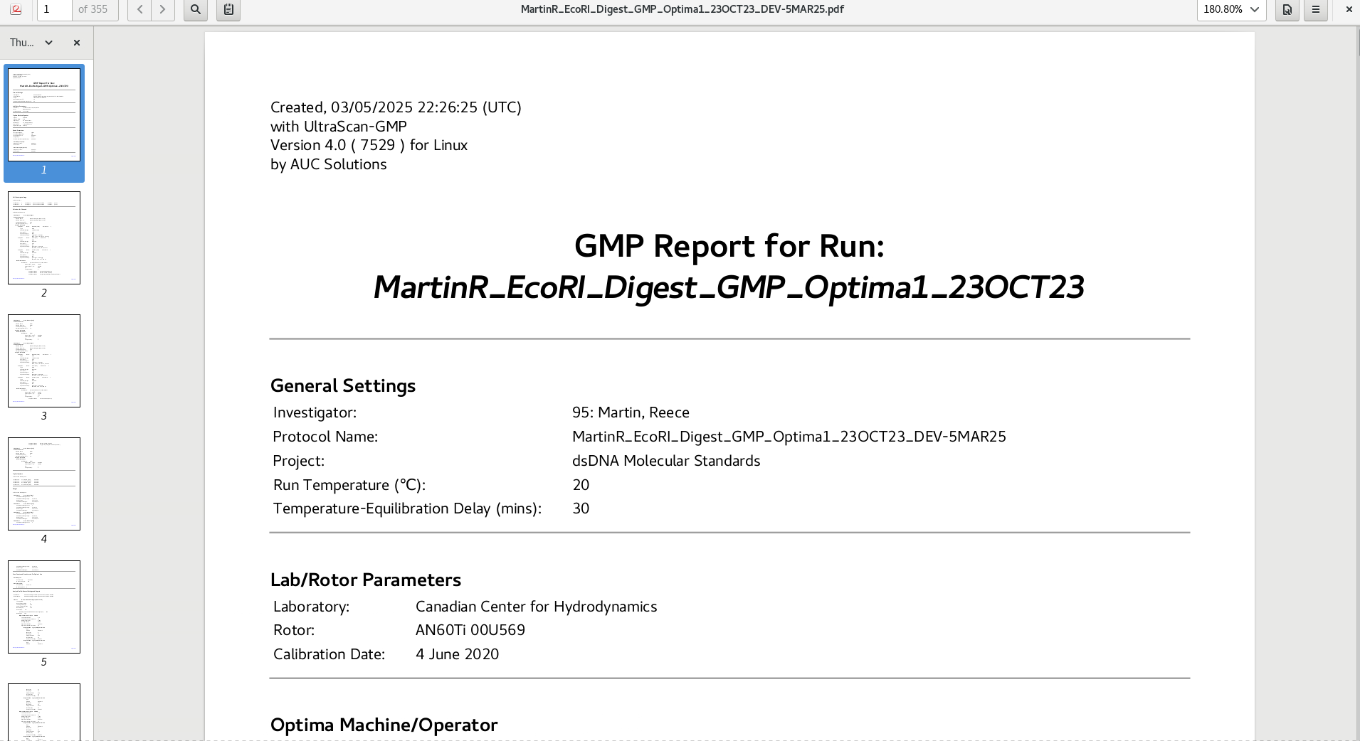
The View Report button opens the PDF file to be viewed: